Elliptic Curve
Mathematics for cryptographic systems
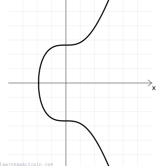
An elliptic curve is used as the basis for some cryptographic systems.
The structure of the elliptic curve allows you to perform a mathematical function ("multiply") to move around the points on the curve in one direction, without being able to travel in the reverse direction. This is known as a "trapdoor function", and it's the key feature of elliptic curves that makes them ideal for use in public key cryptography.
So in short, elliptic curves have mathematical properties that make them useful for cryptography, and they're part of the digital signature system used in Bitcoin (ECDSA).
- You don't need to know about elliptic curves to work with Bitcoin, so don't stress yourself with feeling like you need to learn about all this stuff unless you really want to.
- It's safer and easier to use an elliptic curve library in your programming language to handle all of this rather than coding it yourself.
Parameters (Secp256k1)
Satoshi chose the secp256k1 curve for use with ECDSA, which has the following parameters:

 copied
 copied
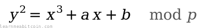
# y² = x³ + ax + b
$a = 0
$b = 7
# prime field
$p = 115792089237316195423570985008687907853269984665640564039457584007908834671663 #=> 2**256 - 2**32 - 2**9 - 2**8 - 2**7 - 2**6 - 2**4 - 1
# number of points on the curve we can hit ("order")
$n = 115792089237316195423570985008687907852837564279074904382605163141518161494337
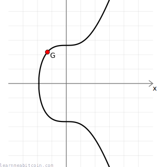
# generator point (the starting point on the curve used for all calculations)
$G = {
x: 55066263022277343669578718895168534326250603453777594175500187360389116729240,
y: 32670510020758816978083085130507043184471273380659243275938904335757337482424,
}
a,b– An elliptic curve is a set of points described by the equationy² = x³ + ax + b, so this is where theaandbvariables come from. Different curves will have different values for these coefficients, anda=0andb=7are the ones specific to secp256k1.p– This is the prime modulus. It's a number that keeps all of the numbers within a specific range when performing mathematical calculations (again it's specific to secp256k1). The fact that it's a prime number is a key ingredient for the cryptography to work.n– This is the order. It's the number of points on the curve that we can reach. It's less thanp, and it's influenced by the chosen generator point (see below).G– This is the generator point. This is the starting point on the curve used when performing most mathematical operations. The exact origin for the choice of this point is unknown, but it's usually because it provides a high order (see above) and has shown to not have any inherent cryptographic weaknesses.
Secp256k1 is just the name for one of the specific elliptic curves used in cryptography. It's short for:
- sec = Standard for Efficient Cryptography — A consortium that develops commercial standards for cryptography.
- p = Prime — A prime number is used to create the finite field.
- 256 = 256 bits — Size of the prime field used.
- k = Koblitz — Specific type of curve.
- 1 = First curve in this category.
Why did Satoshi choose Secp256k1?
I must admit, this project was 2 years of development before release, and I could only spend so much time on each of the many issues. [...] I didn't find anything to recommend a curve type so I just… picked one.
Finite Field
Finite Field – A ring of integers with a finite number of elements.
The diagrams I'm using in this tutorial show a smooth elliptic curve like this:
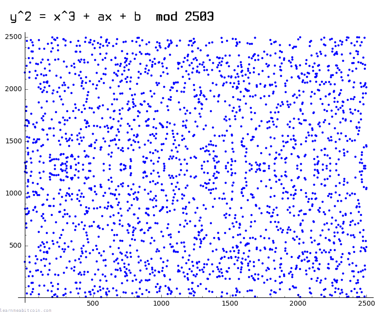
However, the actual curve used in Bitcoin looks more like a scatter plot of points like this:

This is due to the fact that the curve used in Bitcoin is over a finite field of whole numbers (i.e. using mod p to restrict numbers to within a certain range), and this breaks the continuous curve you're able to get when you use real numbers.
However, even though these plots look wildly different, the mathematical operations you can perform on both of these curves still work in the same way.
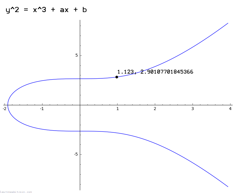
Of course, the secp256k1 curve has a very large value for p, so it more closely resembles the graph below, except imagine there are about as many points on it as there are atoms in the universe:
Sage Math
I made the graphs on this page using Sage Math.
Install on Ubuntu:
sudo apt install sagemathCreate an elliptic curve over a rational field (real numbers):
sage: C = EllipticCurve([0,7]) # y^2 = x^3 + 7, where a=0, b=7
sage: plot(C)
sage: C.lift_x(1.123) # get example y coordinate
sage: C.lift_x(-1.834) # get example y coordinate
Create an elliptic curve over a small finite field:
Sage: F = FiniteField(47)
sage: C = EllipticCurve(F, [0, 7]) # y^2 = x^3 + 7, where a=0, b=7
sage: plot(C)
sage: C.lift_x(17) # get example y coordinate
Create the elliptic curve used in Bitcoin (will be slow):
sage: F = FiniteField(115792089237316195423570985008687907853269984665640564039457584007908834671663)
sage: C = EllipticCurve(F, [0, 7])
Why use a finite field?
Because when implementing cryptography on computers, it's easier to work with the whole numbers in a finite field (e.g. 1, 2, 3, 4, ..., p) than it is to work with an infinite amount of the real numbers (e.g. 0.911722707844879, 2.90107701845366, ...).
You risk losing accuracy when working with decimal numbers on a computer, so the precision you get with a finite set of whole numbers is better suited for cryptography.
For illustrative purposes I'll use the smooth curve for the rest of this tutorial.
Elliptic Curve Mathematics
There are a few mathematical operations that you can perform on points on the elliptic curve. The two main operations are double() and add(), and these can then be combined to perform multiply().
These operations are the building blocks of elliptic curve cryptography, and are used for generating public keys and signatures in ECDSA.
Modular Inverse
Before we can perform the double() and add() operations on points on the curve, we first need to be able to find the modular inverse of a number in a finite field.
The is because the double() and add() equations include the division / operation.
However, there is no straightforward division operation within a finite field of numbers. Instead, you can multiply by the inverse of a number to achieve the same result as division:
In other words, if you start at a specific number in a finite field and multiply by another number, you can "go backwards" to the number you started with by multiplying again by the inverse of the number you used for multiplication.
Obviously this is a confusing first step in to elliptic curve math, but just think of "multiplying by the inverse" as a replacement for division in modular arithmetic.
This always works if you have a prime number of elements in the finite field. A prime number cannot be divided by any other number, so it will distribute the results from modular multiplication back across each of the numbers in the field evenly (without repeating or missing some numbers). So by using a prime number as the modulus, you can guarantee that each number in the finite field will have a multiplicative inverse (or a "division" operation).
So the first step in elliptic curve mathematics is to be able to find the inverse of a number in a finite field:
Code
copiedcopieddef inverse(a, m = $p)

  # store original modulus
  m_orig = m

  # make sure a is positive
  if a < 0
    a = a % m
  end

  # set initial values before loop
  y_prev = 0
  y = 1

  while a > 1
    q = m / a

    y_before = y # store current value of y
    y = y_prev - q * y # calculate new value of y
    y_prev = y_before # set previous y value to the old y value

    a_before = a # store current value of a
    a = m % a # calculate new value of a
    m = a_before # set m to the old a value
  end

  return y % m_orig
end
- This function uses the extended Euclidean algorithm (you don't need to know how it works) to find the modular inverse of a number. It's just a quicker method than trying to find the inverse via brute-force.
- Not all programming languages have a built-in "modular inverse" function, which is why you sometimes have to implement one yourself to get started with elliptic curve mathematics.
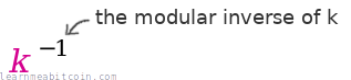
Modular inverse notation
The modular inverse of a number is typically denoted by ⁻¹ in mathematical equations.
In the upcoming operations, the inverse of a number is sometimes found mod p (modulo the prime number), and is sometimes found mod n (modulo the number of points on the curve).
Double
"Doubling" a point is the same thing as "adding" a point to itself.
From a visual perspective, to "double" a point you draw a tangent to the curve at the given point, then find the point on the curve this line intersects (there will only be one), then take the reflection of this point across the x-axis.
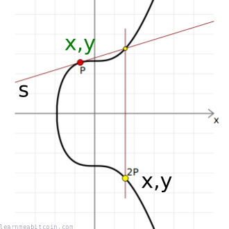
P is a general point on the curve.s refers to the slope of the tangent.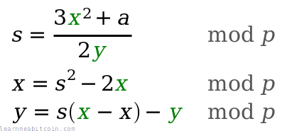
Code
copiedcopieddef double(point)
  # slope = (3x₁² + a) / 2y₁
  slope = ((3 * point[:x] ** 2 + $a) * inverse((2 * point[:y]), $p)) % $p # using inverse to help with division

  # x = slope² - 2x₁
  x = (slope ** 2 - (2 * point[:x])) % $p

  # y = slope * (x₁ - x) - y₁
  y = (slope * (point[:x] - x) - point[:y]) % $p

  # Return the new point
  return { x: x, y: y }
end
Elliptic Curve Operations.
You're not actually "doubling" the values of the x and y coordinates of a point here (like you would do in everyday arithmetic).
The "double", "add", and "multiply" terms on this page refer to specific operations we perform with points on elliptic curves. So even though they have the same names as normal mathematical operations, they are completely different in the domain of elliptic curve mathematics.
This can get a bit confusing at times because there are also everyday "add" and "multiply" operations in amongst these equations too. The trick is to remember that:
- When one of these operations is on a point, we're using the elliptic curve operations.
- When one of these operations is on two integers, it's just everyday arithmetic.
Add
As expected, "addition" of two points in elliptic curve mathematics isn't the same as straightforward integer addition, but it's called "addition" anyway.
From a visual perspective, to "add" two points together you draw a line between them, then find the point on the curve this line intersects (there will only be one), then take the reflection of this point across the x-axis.

Q is a second general point on the curve.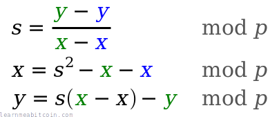
Code
copiedcopieddef add(point1, point2)
  # double if both points are the same
  if point1 == point2
    return double(point1)
  end

  # slope = (y₁ - y₂) / (x₁ - x₂)
  slope = ((point1[:y] - point2[:y]) * inverse(point1[:x] - point2[:x], $p)) % $p

  # x = slope² - x₁ - x₂
  x = (slope ** 2 - point1[:x] - point2[:x]) % $p

  # y = slope * (x₁ - x) - y₁
  y = ((slope * (point1[:x] - x)) - point1[:y]) % $p

  # Return the new point
  return { x: x, y: y }
end
Multiply
This operation is the heart of elliptic curve cryptography.
Most multiplication operations in ECDSA start at the generator point G.
Now that we can double() and add() points on the curve, we can now take any point on the curve and multiply() it by an integer to get to a completely new point.
The simplest method for elliptic curve multiplication would be to repeatedly add() a point to itself until you reach the number you want to multiply by, which would work, but these incremental add() operations would make this approach impossibly slow when multiplying by large numbers (like the ones used in Bitcoin).
Thankfully, there is a faster way to perform multiplication on elliptic curves…
Double-and-add algorithm
3P = 2P + P (one double, one add)A faster approach to multiplication is to use the double-and-add algorithm.
This algorithm uses both doubling and adding to reach the target multiple in as few operations as possible.
For example, if you start at 2 and want to get to 128, it's faster to perform six double() operations than it is to perform sixty-four add() operations.
But how do you know how many double and add operations you need to get to your target multiple?
Well, amazingly, if you convert any integer into its binary representation, the 1s and 0s will provide a map for the sequence of double() and add() operations you need to perform to reach that multiple.
For example:
e.g. 1 * 21

21 = 10101 (binary)
      │││└ double and add = 21
      ││└─ double         = 10
      │└── double and add = 5
      └─── double         = 2
                            1  <- start here
- You always work from left to right.
- You always ignore the first digit.
- You always start with a
double()operation no matter what. This is because you're starting with a single point (e.g. the generator point), so you haven't got two points to add together yet. 0= double1= double and add
Anyway, here's what elliptic curve multiplication looks like when using the double-and-add algorithm in Ruby code:
Code
copiedcopieddef multiply(k, point = $G)
  # create a copy the initial starting point (for use in addition later on)
  current = point

  # convert integer to binary representation
  binary = k.to_s(2)

  # double and add algorithm for fast multiplication
  binary.split("").drop(1).each do |char| # from left to right, ignoring first binary character
    # 0 = double
    current = double(current)

    # 1 = double and add
    current = add(current, point) if char == "1"
  end

  # return the final point
  current
end
Summary
This article just covers the basic mathematical operations used on elliptic curves.
- Finding the modular inverse is a basic requirement for being able to perform the
double()andadd()operations. - The
double()andadd()operations are just building blocks for themultiply()operation. - The
multiply()operation is the core operation used in cryptographic systems.
It's important to remember that "multiplication" on the elliptic curve is nothing like everyday multiplication. It's best to think of "elliptic curve multiplication" as a completely unique kind of operation, but we just call it "multiply" so that it has its own name. It's just unfortunate that it's so confusing.
Anyway, this multiply() operation allows you to move around points on the curve in one direction, but there is no mathematical operation that allows you to "undo" this movement, and this property is what makes elliptic curves so useful for cryptography.
All of this elliptic curve mathematics is used as the basis for the digital signature systems used in Bitcoin: ECDSA and Schnorr (added in 2021 as part of the Taproot upgrade).
Resources
References:
- sec2-v2.pdf – List of recommended curves for use in elliptic curve cryptography from SECG. Contains parameters for the secp256k1 curve used in Bitcoin.
Explanations:
- Elliptic Curve Cryptography: A Gentle Introduction – An excellent four-part introduction to Elliptic Curve Cryptography by Andrea Corbellini. A good place to start.
- Introducing Elliptic Curves – Introduction to elliptic curves by someone who has a deep understanding of why they are used in cryptography.
- An Introduction to Elliptic Curve Cryptography – Another introduction to ECC. Shorter than the two guides above, but I found it helpful.
Tools:
- Elliptic Curve Plotter – A small but cool program that allows you to play with simple elliptic curve operations. It's what I used to help create the diagrams on this page.
- Sage Math – A big mathematical library that comes with elliptic curve plotting functions. I used it to show the plots of elliptic curves over real numbers and over finite fields.
- Interactive Elliptic Curve Operations – A cool web tool created by Andrea Corbellini that allows you to visualise elliptic curve addition and double operations over both real numbers and a finite field.